3. Tutorial

3.1. Automatic Differentiation

Fundamental of automatic differentiation (AD) is the decomposition of differentials based on the chain rule. Qualia implements the reverse accumulation AD in qualia2.autograd.

import qualia2

[*] GPU acceleration enabled.
-----------------------------------------------------------------------
nvcc: NVIDIA (R) Cuda compiler driver
Copyright (c) 2005-2019 NVIDIA Corporation
Built on Fri_Feb__8_19:08:17_PST_2019
Cuda compilation tools, release 10.1, V10.1.105

-----------------------------------------------------------------------

Qualia uses the so called “Define-by-Run” scheme, so forward computation itself defines the computational graph. By using a Tensor object, Qualia can keep track of every operation. Here, the resulting y is also a Tensor object, which points to its creator(s).

x = qualia2.array([5])
y = x**2 - 2*x + 1
print(y)

[16.] shape=(1,)

At this moment we can compute the derivative.

y.backward()
print(x.grad)

[8.]

Note that this meets the result of symbolic differentiation.

All these computations can be generalized to a multidimensional tensor input. When the output is not a scalar quantity, a tenspr with the same dimentions as the output that is filled with ones will be given by default to start backward computation.

x = qualia2.array([[1, 2, 3], [4, 5, 6]])
y = x**2 - 2*x + 1
y.backward()
print(x.grad)

[[ 0.  2.  4.]
 [ 6.  8. 10.]]

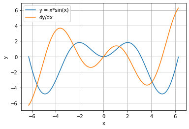
With the autograd feature of Qualia, one can plot the derivative curve of a given function very easily. For instance, let function of interest be y = x*sin(x). Note that the qualia array needs to be converted to numpy array before the plot.

from qualia2.functions import sin
import matplotlib.pyplot as plt

x = qualia2.arange(-2*qualia2.pi,2*qualia2.pi,0.01)
y = x * sin(x)
y.backward()

plt.plot(x.asnumpy(), y.asnumpy(), label='y = x*sin(x)')
plt.plot(x.asnumpy(), x.gradasnumpy(), label='dy/dx')
plt.xlabel('x')
plt.ylabel('y')
plt.legend(loc='upper left')
plt.grid()

plt.show()

3.2. Validation of Automatic Differentiation

One can use util.check_function() to validate the gradient caluclation of a function. util.check_function() internally calculates the gradient using numerical method and compares the result with automatic differentiation. One can specify the domain to avoid null value for the function that has not defined region.

from qualia2.functions import *
from qualia2.util import check_function

grad, sse = check_function(tan, domain=(-np.pi/4, np.pi/4))

[*] measured error: 1.073802239416379e-12

One can use util.check_function() to validate the user defined function. Also, one can specify the input x to check the gradient at given x.

def func(x):
    return x*sin(x)-5*x**2+cos(x)+x

print('auto_grad:{}, numerical_grad:{}'.format(*check_function(func, x=qualia2.array(2))[0]))

[*] measured error: 2.8106903877255435e-18

auto_grad:[-19.83229367], numerical_grad:[-19.83229367]

3.3. Qualia Tensor

Every tensor calculation and automatic differentiation are done by the Tensor onject in Qualia. Tensor onject wraps ndarray objects along the creator onject to perform automatic differentiation. A computational graph for a differentiation is defined dynamically as program runs.

x = qualia2.array([[1, 2, 3], [4, 5, 6]])
print(type(x))
print(x)

<class 'qualia2.autograd.Tensor'>
[[1. 2. 3.]
 [4. 5. 6.]] shape=(2, 3)

The gradient for a Tensor can be optionally replaced by a new gradient, which is additionally calculated by a hooked function.

a = qualia2.rand(5,6)
a.backward()
print(a.grad)

[[1. 1. 1. 1. 1. 1.]
 [1. 1. 1. 1. 1. 1.]
 [1. 1. 1. 1. 1. 1.]
 [1. 1. 1. 1. 1. 1.]
 [1. 1. 1. 1. 1. 1.]]

If lambda grad: 2*grad is registered as a hook, the gradient will be doubled.

a = qualia2.rand(5,6)
a.register_hook(lambda grad: 2*grad)
a.backward()
print(a.grad)

[[2. 2. 2. 2. 2. 2.]
 [2. 2. 2. 2. 2. 2.]
 [2. 2. 2. 2. 2. 2.]
 [2. 2. 2. 2. 2. 2.]
 [2. 2. 2. 2. 2. 2.]]

3.4. Tensor-Numpy Conversion

Numpy ndarray can be used to create the Tensor.

import numpy as np

n = np.arange(18).reshape(3,6)
a = qualia2.autograd.Tensor(n)

print(type(a))
print(a)

<class 'qualia2.autograd.Tensor'>
[[ 0.  1.  2.  3.  4.  5.]
 [ 6.  7.  8.  9. 10. 11.]
 [12. 13. 14. 15. 16. 17.]] shape=(3, 6)

Tensor can be easily converted to numpy ndarray by using Tensor.asnumpy(). Note that resulting ndarray does not carry any of the gradient information.

b = a.asnumpy()

print(type(b))
print(b)

<class 'numpy.ndarray'>
[[ 0.  1.  2.  3.  4.  5.]
 [ 6.  7.  8.  9. 10. 11.]
 [12. 13. 14. 15. 16. 17.]]

3.5. Computational Graph

If you want to detach the computation from the current graph, you can use Tensor.detach() method. This will clear the creator object in the Tensor and prevents backward propagation to be computed further.

from qualia2.functions import *

a = qualia2.rand(5,6)
b = sin(a)

b.backward()
print(a.grad)

[[0.76790906 0.71244082 0.83183156 0.96897591 0.64806117 0.75165602]
 [0.82414905 0.58799685 0.96589815 0.67495328 0.95247465 0.93182726]
 [0.89724121 0.98999407 0.77401058 0.99550057 0.98964091 0.80678068]
 [0.98992852 0.69552181 0.73793413 0.99660953 0.63206233 0.60313844]
 [0.59003014 0.81016324 0.84843595 0.616491   0.74049448 0.92092612]]

a = qualia2.rand(5,6)
b = sin(a).detach()

b.backward()
print(a.grad)

None

3.6. Network Definition

In order to define a network, nn.Module needs to be inherited. Note that a user-defined model must have super().__init__() in the __init__ of the model.

import qualia2.nn as nn
import qualia2.functions as F

class Model(nn.Module):
    def __init__(self):
        super().__init__()
        self.conv1 = nn.Conv2d(1, 10, kernel_size=5)
        self.conv2 = nn.Conv2d(10, 20, kernel_size=5)
        self.fc1 = nn.Linear(500, 50)
        self.fc2 = nn.Linear(50, 10)

    def forward(self, x):
        x = F.relu(F.maxpool2d(self.conv1(x), (2,2)))
        x = F.relu(F.maxpool2d(self.conv2(x), (2,2)))
        x = F.reshape(x,(-1, 500))
        x = F.relu(self.fc1(x))
        x = self.fc2(x)
        return x

model = Model()

If the model is sequential, there is also an option to use nn.Sequential.

model = nn.Sequential(
    nn.Conv2d(1, 10, kernel_size=5),
    nn.MaxPool2d((2,2)),
    nn.ReLU(),
    nn.Conv2d(10, 20, kernel_size=5),
    nn.MaxPool2d((2,2)),
    nn.ReLU(),
    nn.Flatten(),
    nn.Linear(500, 50),
    nn.ReLU(),
    nn.Linear(50, 10),
)

3.7. Model Summary

Having a visualization of the model is very helpful while debugging your network. You can obtain a network summary by your_model.summary(input_shape). Note that the input_size is required to make a forward pass through the network.

model = Model()
model.summary((1, 1, 28, 28))

----------------------------------------------------------------------------
                                Model: Model
----------------------------------------------------------------------------
| layers              |    input shape     |    output shape    | params # |
============================================================================
| Conv2d              |   (1, 1, 28, 28)   |  (1, 10, 26, 26)   |   260    |
| Conv2d              |  (1, 10, 13, 13)   |  (1, 20, 11, 11)   |   5020   |
| Linear              |      (1, 500)      |      (1, 50)       |  25050   |
| Linear              |      (1, 50)       |      (1, 10)       |   510    |
============================================================================
total params: 30840
training mode: True
----------------------------------------------------------------------------

3.8. Saving/Loading a Trained Weights

In order to save the trained weights of a model, one can simply use Module.save(filename) method. The weights are saved in pickle format with .qla extension. To load the saved weights, use Module.load(filename) method.

model.save('tutorial_weights')
model.load('tutorial_weights')

3.9. Setting up an Optimizer

Optimizers require the model parameters. Put Module.params as the first argument for the optimizer. Other arguments such as learning rate are optional.

from qualia2.nn.optim import SGD

optim = SGD(model.params)

Following optimizers are available now:

• SGD (Momentum)

• Adagrad

• Adadelta

• RMSProp

• Adam

• AdaMax

• Nadam

• RAdam

• NovoGrad

You can gat the parameters as:

optim.state_dict()

{'lr': 0.001, 'm': 0, 'l2': 0, 'v': {}}

You can change the parameters by passing the dictionary:

optim.load_state_dict({'lr':0.01, 'm': 0.1, 'l2': 0.9})
optim.state_dict()

{'lr': 0.01, 'm': 0.1, 'l2': 0.9, 'v': {}}

3.10. Dataloader

Dataloader is the user friendly class that helps the preprocess of data for training, testing, and visualization purpose. One can create the customized DatalLoader by just defining:

• self.train_data

• self.train_label

• self.test_data

• self.test_label

Note that if you do not have some of the properties above, you can leave it as None. Also, if you need to visualize the data, overrite DataLoader.show() method.

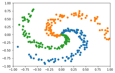
Here is the example of creating a spiral data.

from qualia2.data.dataloader import DataLoader

class Spiral(DataLoader):
    '''Spiral Dataset\n
    Args:
        num_class (int): number of classes
        num_data (int): number of data for each classes

    Shape:
        - data: [num_class*num_data, 2]
        - label: [num_class*num_data, num_class]
    '''
    def __init__(self, num_class=3, num_data=100):
        super().__init__()
        self.num_class = num_class
        self.num_data = num_data
        self.train_data = np.zeros((num_data*num_class, 2))
        self.train_label = np.zeros((num_data*num_class, num_class))

        for c in range(num_class):
            for i in range(num_data):
                rate = i / num_data
                radius = 1.0*rate
                theta = c*4.0 + 4.0*rate + np.random.randn()*0.2
                self.train_data[num_data*c+i,0] = radius*np.sin(theta)
                self.train_data[num_data*c+i,1] = radius*np.cos(theta)
                self.train_label[num_data*c+i,c] = 1

    def show(self, label=None):
        fig, ax = plt.subplots()
        for c in range(self.num_class):
            ax.scatter(self.train_data[(self.train_label[:,c]>0)][:,0],self.train_data[(self.train_label[:,c]>0)][:,1])
        plt.xlim(-1,1)
        plt.ylim(-1,1)
        plt.show()

Let’s visualize the spiral data we just created.

data = Spiral()
data.show()

[*] preparing data...
    this might take few minutes.

DataLoader yields shuffuled mini-batch data for every iteration. Batch size can be set as follows:

data.batch = 100
feat, label = next(data)
print(feat.shape)

(100, 2)

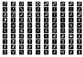
Dataloaders for famous datasets such as MNIST are provided in qualia2.data. One can simply use a dataset by importing the DataLoader for the dataset.

from qualia2.data import MNIST

data = MNIST()

[*] preparing data...
[*] done.

data.show()

3.11. Qualia2 Vision

Qalia2 vision provides some pretrained models for computer vision tasks. Following models are available with pretrained weights now:

• AlexNet

• VGG

• ResNet

• SqueezeNet

• DenseNet

• OpenPose

import qualia2.vision as qualiavision

To load the model:

model = qualiavision.VGG11(pretrained=False)

The model structure can be printed by repr.

model

VGG(
    [0] features: Sequential(
    [0] 0: Conv2d(3, 64, (3, 3), stride=(1, 1), padding=(1, 1), dilation=(1, 1), bias=True) at 0x00007F3768736C88
    [1] 1: ReLU() at 0x00007F37687364E0
    [2] 2: MaxPool2d((2, 2), stride=(2, 2), padding=(0, 0), dilation=(1, 1), return_indices=False) at 0x00007F3768736BE0
    [3] 3: Conv2d(64, 128, (3, 3), stride=(1, 1), padding=(1, 1), dilation=(1, 1), bias=True) at 0x00007F3768736E80
    [4] 4: ReLU() at 0x00007F3768736828
    [5] 5: MaxPool2d((2, 2), stride=(2, 2), padding=(0, 0), dilation=(1, 1), return_indices=False) at 0x00007F3768736160
    [6] 6: Conv2d(128, 256, (3, 3), stride=(1, 1), padding=(1, 1), dilation=(1, 1), bias=True) at 0x00007F3768736E48
    [7] 7: ReLU() at 0x00007F37687366A0
    [8] 8: Conv2d(256, 256, (3, 3), stride=(1, 1), padding=(1, 1), dilation=(1, 1), bias=True) at 0x00007F37687368D0
    [9] 9: ReLU() at 0x00007F3768736940
    [10] 10: MaxPool2d((2, 2), stride=(2, 2), padding=(0, 0), dilation=(1, 1), return_indices=False) at 0x00007F37687362E8
    [11] 11: Conv2d(256, 512, (3, 3), stride=(1, 1), padding=(1, 1), dilation=(1, 1), bias=True) at 0x00007F3768736588
    [12] 12: ReLU() at 0x00007F3768736240
    [13] 13: Conv2d(512, 512, (3, 3), stride=(1, 1), padding=(1, 1), dilation=(1, 1), bias=True) at 0x00007F37687365C0
    [14] 14: ReLU() at 0x00007F3768736630
    [15] 15: MaxPool2d((2, 2), stride=(2, 2), padding=(0, 0), dilation=(1, 1), return_indices=False) at 0x00007F37687365F8
    [16] 16: Conv2d(512, 512, (3, 3), stride=(1, 1), padding=(1, 1), dilation=(1, 1), bias=True) at 0x00007F3768736358
    [17] 17: ReLU() at 0x00007F3768736400
    [18] 18: Conv2d(512, 512, (3, 3), stride=(1, 1), padding=(1, 1), dilation=(1, 1), bias=True) at 0x00007F3768736048
    [19] 19: ReLU() at 0x00007F3768756630
    [20] 20: MaxPool2d((2, 2), stride=(2, 2), padding=(0, 0), dilation=(1, 1), return_indices=False) at 0x00007F3768756400
) at 0x00007F3768736B70

    [1] classifier: Sequential(
    [0] 0: Linear(25088, 4096, bias=True) at 0x00007F3768756438
    [1] 1: ReLU() at 0x00007F37687561D0
    [2] 2: Dropout(p=0.5) at 0x00007F3768756898
    [3] 3: Linear(4096, 4096, bias=True) at 0x00007F3768756518
    [4] 4: ReLU() at 0x00007F3768756940
    [5] 5: Dropout(p=0.5) at 0x00007F3768756A58
    [6] 6: Linear(4096, 1000, bias=True) at 0x00007F37687569B0
) at 0x00007F3768756B00

) at 0x00007F37687564E0