Denavit–Hartenberg convention
In this convention, coordinate frames are attached to the joints between two links such that one transformation is associated with the joint
where each transformation
def transform(a, alpha, d, theta):
    return Rot(theta, axis="z") @ Trans(d, axis="z") @ Trans(a, axis="x") @ Rot(alpha, axis="x")
Forward Kinematics
Forward kinematics is the problem of finding the end-effector position and orientation
We can use the DH parameters of a robot to simply represent the forward kinematics as a chain of transformations starting from a base link, which connects to the origin.
def fk(theta):
    trans = np.identity(4)
    for (_a, _alpha, _d, _theta) in dh_params(theta):
        trans = trans @ transform(_a, _alpha, _d, _theta)
    return trans
Forward Kinematics
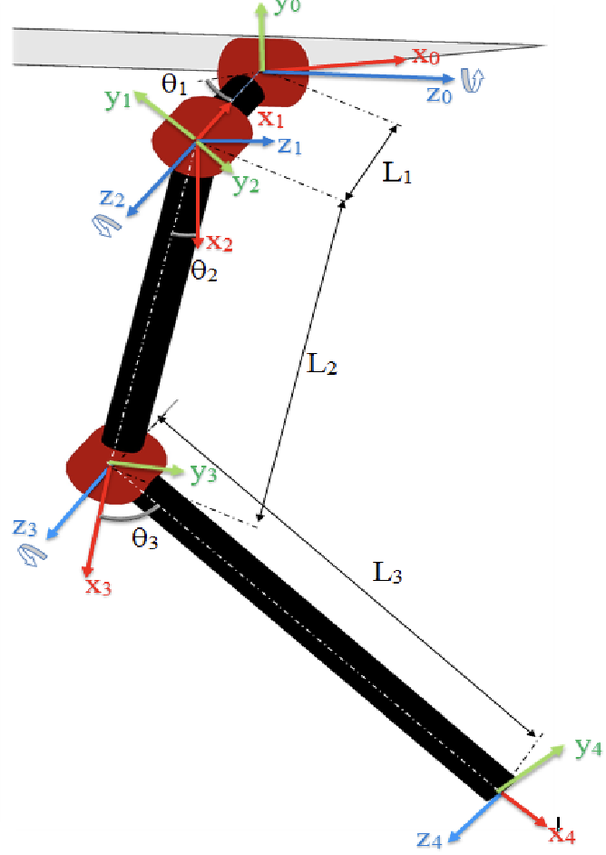
Let's consider the right front leg joints (coordinate systems below):

The DH parameters of the leg:
| Link | ||||
|---|---|---|---|---|
| 0-1 | ||||
| 1-2 | ||||
| 2-3 | ||||
| 3-4 |
From the table, we can construct the each transformation
Inverse Kinematics
Inverse kinematics (IK) is essentially the reverse operation of FK: computing configuration(s) to reach a desired workspace coordinate. Unlike forward kinematics, inverse kinematics cannot be solved in a closed-form expression (in general). If we can derive a closed-form expression through symbolic manipulations, we can use Analytical IK, otherwise we need to use numerical approach.
Analytical IK
- Once the equations are derived, solutions are very fast to compute.
- Often difficult or tedious to derive.
- Only applicable to non-redundant robots (# DOFs = # of task space dimensions).
Numerical IK
- need to define solution parameters or initial guesses
- More generalizable
Analytical Inverse Kinematics
Let's consider a 2D arm in 2D space as in the Figure.
From law of cosines:
Assuming solution exists (
- Note that elbow down and elbow up solutions (
Then using the
Analytical Inverse Kinematics
Given the foot position
where
- the
Jacobian
The Jacobian matrix is a matrix of partial derivatives that describes how the robot's configuration affects the robot's end-effector position. The Jacobian matrix is defined as:
where
If we consider the differentiation w. r. t. time, we can write the relationship between
Basic Jacobian
Numerical Inverse Kinematics
Given an initial guess
where
By truncating the Taylor expansion at first order, we can obtain the approximation as:
Assuming that
- In practice, pseudo-inverse of a Jacobian
We will iteratively update the guess until it converges to a solution.